The Naive Bayes Classifier is a well known machine learning classifier with applications in Natural Language Processing (NLP) and other areas. Despite its simplicity, it is able to achieve above average performance in different tasks like sentiment analysis. Today we will elaborate on the core principles of this model and then implement it in Python. In the end, we will see how well we do on a dataset of 2000 movie reviews. Let’s get started!

Core
The math behind this model isn’t particularly difficult to understand if you are familiar with some of the math notation. For those of you who aren’t, I’ll do my best to explain everything thoroughly. Let’s start with our goal, to correctly classify a review as positive or negative. These are the two classes to which each document belongs.

In more mathematical terms, we want to find the most probable class given a document, which is exactly what the above formula conveys. C is the set of all possible classes, c is one of these classes and d the document that we are currently classifying. We read P(c|d) as the probability of class c, given document d.
We can rewrite this equation using the well known Bayes’ Rule, one of the most fundamental rules in machine learning. Since we want to maximize the equation we can drop the denominator, which doesn’t depend on class c.
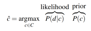
The rewritten form of our classifier’s goal naturally splits it into two parts, the likelihood and the prior. You can think of the latter as “the probability that given a class c, document d belongs to it” and the former as “the probability of having a document from class c”. To go a step further we need to introduce the assumption that gives this model its name.
Naive Bayes assumption: given a class c, the presence of an individual feature of our document is independent on the others.
We consider each individual word of our document to be a feature. If we write this formally we obtain:

The Naive Bayes assumption lets us substitute P(d|c) by the product of the probability of each feature conditioned on the class because it assumes their independence.
We can make one more change: maximize the log of our function instead. The reason for this is purely computational since the log space tends to be less prone to underflow and more efficient. We arrive at the final formulation of the goal of the classifier.

So how exactly does this reformulation help us? Let’s look at each term individually.
-
- P(c) is simply the probability of encountering a document of a certain class within our corpus. This is easily calculated by just dividing the number of occurrences of class c by the total number of documents.
- P(w_i|c) is the probability of word w_i occurring in a document of class c. Again we can use the frequencies in our corpus to compute this. This will simply be the number of times word w_i occurs in documents of class c, divided by the sum of the counts of each word that appears in documents of class c.
We can compute all the terms in our formulation, meaning that we can calculate the most likely class of our test document! There is only one issue that we need to deal with: zero probabilities.
Smoothing
Imagine that you are trying to classify a review that contains the word ‘stupendous’ and that your classifier hasn’t seen this word before. Naturally, the probability P(w_i|c) will be 0, making the second term of our equation go to negative infinity! This is a common problem in NLP but thankfully it has an easy fix: smoothing. This technique consists in adding a constant to each count in the P(w_i|c) formula, with the most basic type of smoothing being called add-one (Laplace) smoothing, where the constant is just 1.

This solves the zero probabilities problem and we will see later just how much it impacts the accuracy of our model.
Implementation
We will implement our classifier in the form of a NaiveBayesClassifier class. We will split the algorithm into two essential parts, the training and classifying.
Training
In this phase, we provide our classifier with a (preferably) large corpus of text, denoted as D, which computes all the counts necessary to compute the two terms of the reformulated.
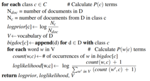
When implementing, although the pseudocode starts with a loop over all classes, we will begin by computing everything that doesn’t depend on class c before the loop. This is the case for N_doc, the vocabulary and the set of all classes.
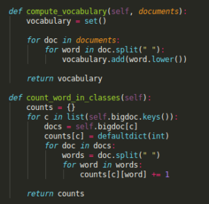
Since the bigdoc is required when computing the word counts we also calculate it before the loop.
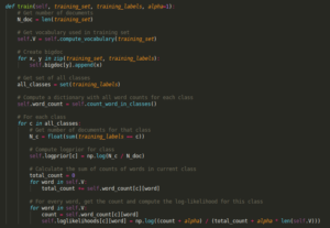
Within the loop, we just follow the order as given in the pseudocode.
-
- First, we count the number of documents from D in class c.
-
- Then we calculate the logprior to that particular class.
-
- Next, we make a loop over our vocabulary so that we can get a total count for the amount of words within class c.
- Finally, we compute the log-likelihoods of each word for class c using smoothing to avoid division-by-zero errors.
Classifying
When the training is done we have all the necessary values to make a prediction. This will simply consist in taking a new (unseen) document and computing the probabilities for each class that has been observed during training.
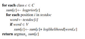
We initialize the sums dictionary where we will store the probabilities for each class. We always compute the probabilities for all classes so naturally the function starts by making a loop over them. For each class c, we first add the logprior, the first term of our probability equation. The second term requires us to loop over all words, and increment the current probability by the log-likelihood of each.
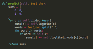
Once this is done, we can just get the key of the maximum value of our dictionary and voilà, we have a prediction. We are now ready to see Naive Bayes in action!
Data
We will test our model on a dataset with 1000 positive and 1000 negative movie reviews. Each document is a review and consists of one or more sentences.
We split the data into a training set containing 90% of the reviews and a test set with the remaining 10%. As the name implies, the former is used for training the model with our train function, while the latter will give us an idea how well the model generalizes to unseen data.
Once that is done, we need some sort of baseline to compare the accuracy of our model with, otherwise, we can’t really tell how good it is doing. Since this is a binary classification task, we at least know that random guessing should net us an accuracy of around 50%, on average. Anything close to this number is essentially random guessing.
Results
Let’s take a look at the full implementation of the algorithm, from beginning to end.

Yes, that’s it! All we had to do was create the classifier, train it and use the validation set to check its accuracy. I omitted the helper function to create the sets and labels used for training and validation. Let’s see how our model does without smoothing, by setting alpha to 0 and running it
Predicted correctly 101 out of 202 (50.0%)
Ran in 1.016 seconds
Eugh.. that’s disappointing. One would expect to do at the very least slightly better than average even without smoothing. Let’s add smoothing
Predicted correctly 167 out of 202 (82.67327%)
Ran in 0.961 seconds
Now that is some accuracy! Smoothing makes our model good enough to correctly classify at least 4 out of 5 reviews, a very nice result. We also see that training and predicting both together take at most 1 second which is a relatively low runtime for a dataset with 2000 reviews.
Conclusion
As we could see, even a very basic implementation of the Naive Bayes algorithm can lead to surprisingly good results for the task of sentiment analysis. Notice that this model is essentially a binary classifier, meaning that it can be applied to any dataset in which we have two categories. There are all kinds of applications for it, ranging from spam detection to bitcoin trading based on sentiment. With an accuracy of 82%, there is really a lot that you could do, all you need is a labeled dataset and of course, the larger it is, the better!
If you are interested in AI, feel free to check out my GitHub: https://github.com/filipkny/MediumRare. I’ll be putting the source code together with the data there so that you can test it out for yourself.
Thank you for reading.
Related Articles:
