In this article, I want to show you how to build a classifier using a Neural Network. The main purpose of this article is to show you how to implement a Neural Network from Scratch in Python using Numpy. You will learn how to implement a neural network from scratch in Python.
Pre-reqs:
I assume that you have basic knowledge of neural networks and you have coded it once either from scratch or using any framework. I also assume that you have familiarity with Numpy and Python. I also assume that you have some knowledge of Machine Learning notations/ commonly used terminologies.
Outcomes:
Implement a Neural Network with a single hidden layer.
Learn how to Compute the cross-entropy loss.
Implement forward and backward propagation
Learning Approach:
We will break all tasks in different pieces and code them in functions. In the end, we will combine everything together in a function known as a model.
Data set:
We will generate our own planar data set and we will classify it using a neural network. Let's generate a dataset using numpy. I won't go into details of how this generation works but if you have good knowledge of maths equations, you will understand it.
.
This code is copied from Deep Learning Specialization by deeplearning.ai to genereate the data set.
Data Visualization:
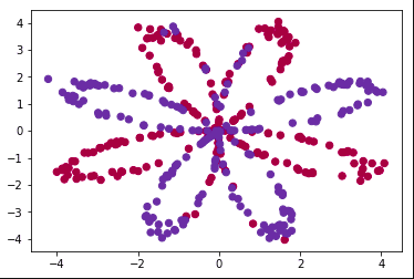
Let's visualize the data set to understand the problem further and to tackle it easily.
X.shape(2,400)
Y.shape(1,400)
plt.scatter(X[0,:], X[1,:],c = Y[0], s=40, cmap=plt.cm.Spectral);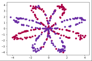
Here we can see that this is a pretty descent classficiation problem where we have to classify read and blue points.
Neural Network Architecture:
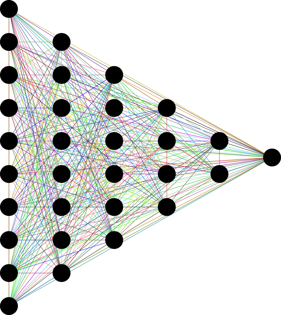
We are going to make a Neural Network with 1 hidden layer having the following architecture.
2 units in the input layer, 4 units in the hidden layer and 1 unit in the output layer. Although it is our choice to change the number of units in hidden layers and the number of hidden layers, but it is a simple task so this simple network will be enough.
Methodology:
We will use a break and conquer rule meaning we will break our task in smaller functions, and then combine them into a larger function using all these tasks. Main methodology we are going to adapt is as follows:
Define the Neural Network structure.
Initialize the model's parameters
Loop to compute Forward Prop, Loss, Back Prop and then update the parameters.
We will make these functions and merge them in the end in the nn_model function compute neural network.
Step # 1 Neural Network Structure:
Remember the structure which is going to have 2 units in the input layer, 4 in hidden and 1 in the output layer. Let's code it.
Here what we are doing is that defining the number of layers and units inside these layers & returning them.
Step # 2 Initialize Parameters
Initializing the parameters correctly has a significant impact on neural network performance. For example, if you initialize the weights of Neural Networks from 0, our model will not perform at all. A general technique to perform initialization is that we pick numbers from a random distribution and multiply it with a small number such as 0.01.
One more thing you need to know about weights initialization is that general formula for (number of weights in layer X = number of units in layer X, a number of units in layer X-1). Let's say for layer number 1, the shape of weights will be (numbers of units in layer # 1, numbers of units in layer # 0).
The general shape of bias in layer X is (number of units in layer X, 1)
Note that either we initialize bias to 0 or to a random number, it does not affect the performance of the neural network. We collected all the parameters in a dictionary known as parameters and returned it. We will use this dictionary in our further tasks and it will help us later.
Activation Function:
For the hidden layer, we will use tanh which is a commonly used activation function, though we can use ReLU(and it will give somewhat better results). For the output layer, we will use sigmoid activation function.
Step # 3 Loop
Now we will compute the functions we will need inside the loop. We will start by computing Forward Propagation
Remember prediction in a neural network is dot product of weights and input units. Then we use activation function on the answer( tanh in our case). Basically we are creating a computational graph here step by step.
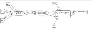 Computational Graph
Now if we keep this computational graph in mind, Computing Backpropagation will be an easy step for us. Think of all arrows in forward direction as Forward Propagation, all Arrows in backwards direction are of backpropagation, where we will take derivatives using the chain rule. Let's compute cost function first and then we will go towards the Backpropagation step.
Cost Function:
The general equation for cost function for binary classification is known as the cross-entropy loss function. Read more about it here. So basically our goal is to compute the cost of the final output and then using backpropagation update the parameters i.e weight and bias.
Backpropagation:
It is indeed the hardest thing in neural networks for most of the people but remembers the computational graph in mind. What we do basically is we compute gradients using the computational graph from loss till our weights and bias, and update them. It is a whole topic and I encourage you to read this article to understand in-depth how backpropagation works. In our case, we are going to have 6 main equations to update. I will write to them first, then explain them and then we will code them.
dZ2= A2 - Y
dW2 = (1 / m) * (dZ2**.**A1)
db2 = (1 / m) * sum(dZ2)
dZ1 = (W2 . dZ2) * (1 - A1^2)
dW1 = (1 / m) * (dZ1 . X)
db1 = (1 / m) * sum(dZ1)
Note that " . " in above equations mean dot product of 2 elements.
Here dZ2 means derivate of Z2 w.r.t cost, dW2 means derivatives of W2 w.r.t cost and so on. Now if you have read the articles and compute the derivates of the equations of the forward propagations in the computational graph shown above yourselves, then you will get the same equations. So basically each equation is the derivate w.r.t cost function we computed. Our goal is to compute the derivatives of weights and bias, and in order to calculate them, we need to calculate the derivates of all the functions as shown above because of these functions lye in a computational graph or chained in each other. We use the popular chain rule to calculate the derivatives.
We store each gradient in a dictionary called grads so that we can retrieve it later on when updating the parameters.
Update Parameters:
Now we are in one of the last steps of our Loop which is to update parameters using Gradients computed using Backpropagation. Our goal is to update and tune W1, W2, b1, and b2 so that our network is trained and performs well. The general way to update parameters is Weight = Weight - (learning rate)*(derivative of Weight) and bias = bias - (learningrate * derivative of bias). Normally the value of the learning rate is small(0.01,0.001 etc.) as we do not want our model to take big steps and instead of improving, it becomes worse.
Here we are storing the updated models in the same dictionary parameters which we passed in our function.
Creating Model:
This marks us to our final step where we will integrate all our helper functions and create a model.
Prediction Phase:
After we have trained our model, we want to know the outputs and to do this we need to predict the outcome of the last node of the model. We will predict that if the output of A2(last node) is greater then 0.5, it is 1(true) else it is 0.
Running Model:
Lets now run the model. Using model function we will run the model.
parameters = model(X, Y, n_h = 4, num_iterations = 10000, print_cost=True)Visualize Data:
In order to visualize the result, we will plot the data and decision boundary using our predict function. Let's make a function for plotting decision boundaries.
Again this code to visualize data by drawing decesion boundary is used in Deep Learning Specialization by deepleanring.ai.
Call this function to check the plotted boundary.
plot_decision_boundary(lambda x: predict(parameters, x.T), X, Y.ravel())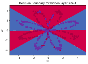 Decision Boundary
We can see that our model has almost classified all the points correctly. This is pretty good progress for a single layer network using the tanh activation function. If we use the ReLU function, and more hidden layers with more number of epochs, we can achieve even better results.
Accuracy:
In order to calculate accuracy, we will again use the predict function and compare it with the original data set to check how it performs.
We can see that our model almost achieved 90% accuracy which is pretty good. I will write some suggestions to improve this accuracy which are
Adding more hidden units
Increasing number of epochs
Adding Regularization term
Changing activation to tanh
There are definitely other ways too to increase the accuracy but these are some of the common ways to increase the accuracy.
Recap:
Let's recap the whole process step by step for a better understanding.
Define the structure of your model.
Initialize your weights and bias
Compute Forward Propagation on all units.
Compute backward propagation to get gradients.
Use gradients computed by backpropagation to update weights and bias.
Combine all these functions in a model function and integrate the functionality.
Predict label 1 if the last layer has output >= 0.5 and label 0 otherwise.
Plot the decision boundaries to check your model.
Learn more about Deep Learning:
This article is inspired by Deep Learning Specialization by deeplearning.ai at Coursera. In order to learn more about deep learning, it is encouraged to complete this specialization.
Image Credits:
Starting Picture: Pixabay In-Post Pictures + Featured Images: Taken by Author